1 | import itertools |
1 | def plot_2d(data, title, figsize=(18,5)): |
原理
- $k$:k 天前
- $r_k$:k 天前新用户第 k 日留存
- $s_k$:k 天前新用户占比
- $K$:历史新老用户分解线,比如将2019年前所有用户当做老用户,之后的新用户看做是新用户
数据
1 | def get_dau(path='./data/0610_dau.xlsx', usecols=['f_date', 'dau'], index_col=0, parse_dates=['f_date']): |
小程序 DAU
1 | dau = get_dau() |
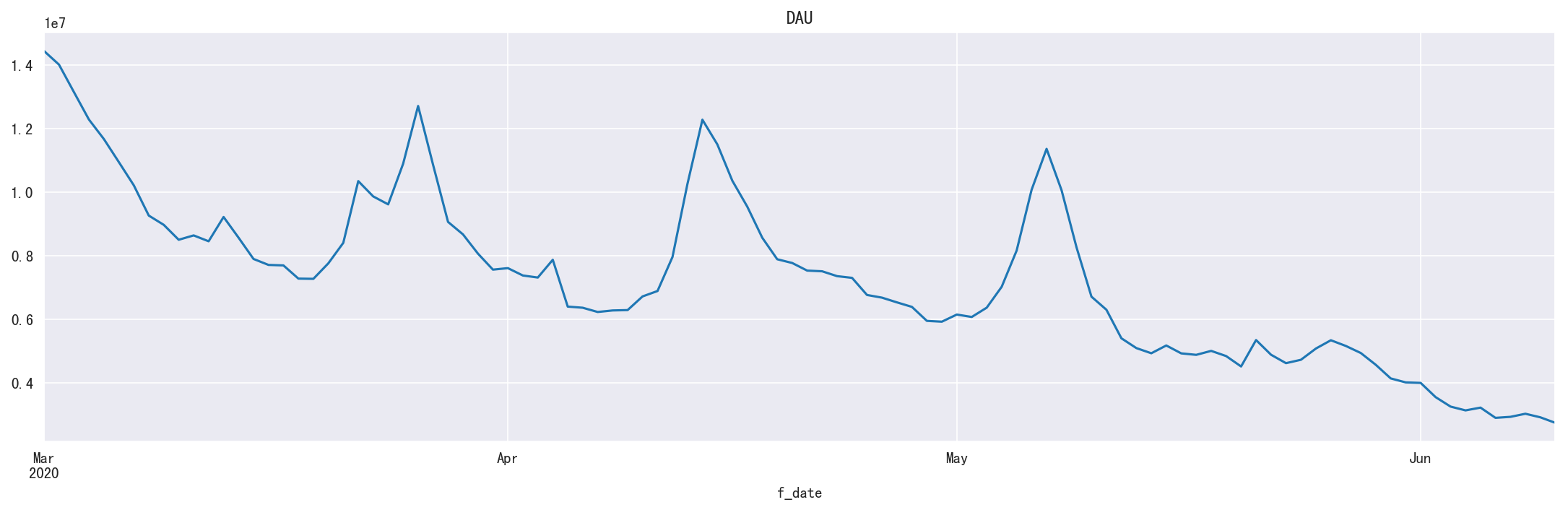
1 | df_show(dau, 10, 10) |
shape=(524,)

f_date
2019-01-04       2960
2019-01-05       2318
2019-01-06       2274
2019-01-07       2601
2019-01-08       2520
2019-01-09       2514
2019-01-10       2315
2019-01-11       2179
2019-01-12       1947
2019-01-13       1813
2020-06-01    3994272
2020-06-02    3546456
2020-06-03    3248834
2020-06-04    3129509
2020-06-05    3216982
2020-06-06    2895258
2020-06-07    2926685
2020-06-08    3023940
2020-06-09    2911481
2020-06-10    2737987
Name: dau, dtype: int64
新增用户
1 | s_dau_new = get_dau_new() |
shape=(161,)


f_date
2020-01-01    183431
2020-01-02    175389
2020-01-03    172991
2020-01-04    157629
2020-01-05    158287
2020-06-05    440420
2020-06-06    419283
2020-06-07    409955
2020-06-08    422092
2020-06-09    412235
Name: f_dau_new, dtype: int64
1 | # '2020-03-01': |

新用户留存
1 | df_ret_new = get_retention_new() |
shape=(160, 120)
| f_remain_days | 1 | 2 | 3 | 4 | 5 | 6 | 7 | 8 | 9 | 10 | ... | 111 | 112 | 113 | 114 | 115 | 116 | 117 | 118 | 119 | 120 |
|---|---|---|---|---|---|---|---|---|---|---|---|---|---|---|---|---|---|---|---|---|---|
| f_visit_day | |||||||||||||||||||||
| 2020-01-01 | 0.02 | 0.01 | 0.01 | 0.01 | 0.01 | 0.01 | 0.01 | 0.01 | 0.00 | 0.01 | ... | 0.01 | 0.01 | 0.01 | 0.01 | 0.01 | 0.01 | 0.01 | 0.01 | 0.01 | 0.01 |
| 2020-01-02 | 0.02 | 0.01 | 0.01 | 0.01 | 0.01 | 0.01 | 0.01 | 0.01 | 0.01 | 0.01 | ... | 0.01 | 0.01 | 0.01 | 0.01 | 0.01 | 0.01 | 0.01 | 0.01 | 0.01 | 0.01 |
| 2020-01-03 | 0.02 | 0.01 | 0.01 | 0.01 | 0.01 | 0.01 | 0.01 | 0.01 | 0.01 | 0.01 | ... | 0.01 | 0.01 | 0.01 | 0.01 | 0.01 | 0.01 | 0.01 | 0.01 | 0.01 | 0.01 |
| 2020-01-04 | 0.02 | 0.01 | 0.01 | 0.01 | 0.01 | 0.01 | 0.01 | 0.01 | 0.01 | 0.01 | ... | 0.01 | 0.01 | 0.01 | 0.01 | 0.01 | 0.01 | 0.01 | 0.01 | 0.01 | 0.01 |
| 2020-01-05 | 0.02 | 0.01 | 0.01 | 0.01 | 0.01 | 0.01 | 0.01 | 0.01 | 0.01 | 0.01 | ... | 0.01 | 0.01 | 0.01 | 0.01 | 0.01 | 0.01 | 0.01 | 0.01 | 0.01 | 0.01 |
| 2020-06-04 | 0.04 | 0.02 | 0.01 | 0.01 | 0.01 | nan | nan | nan | nan | nan | ... | nan | nan | nan | nan | nan | nan | nan | nan | nan | nan |
| 2020-06-05 | 0.04 | 0.02 | 0.01 | 0.01 | nan | nan | nan | nan | nan | nan | ... | nan | nan | nan | nan | nan | nan | nan | nan | nan | nan |
| 2020-06-06 | 0.03 | 0.02 | 0.01 | nan | nan | nan | nan | nan | nan | nan | ... | nan | nan | nan | nan | nan | nan | nan | nan | nan | nan |
| 2020-06-07 | 0.03 | 0.02 | nan | nan | nan | nan | nan | nan | nan | nan | ... | nan | nan | nan | nan | nan | nan | nan | nan | nan | nan |
| 2020-06-08 | 0.04 | nan | nan | nan | nan | nan | nan | nan | nan | nan | ... | nan | nan | nan | nan | nan | nan | nan | nan | nan | nan |
10 rows × 120 columns
1 | df_ret_new_plot = df_ret_new.loc['2020-02-10':] |

老用户留存
1 | s_ret_old = get_retention_old() |
shape=(101,)


f_date
2020-03-01   0.05
2020-03-02   0.05
2020-03-03   0.04
2020-03-04   0.04
2020-03-05   0.04
2020-06-05   0.01
2020-06-06   0.01
2020-06-07   0.01
2020-06-08   0.01
2020-06-09   0.01
Name: f_ratio, dtype: float64
1 | plot_2d(s_ret_old,u'老用户留存') |
模型
1 |
|
1 | base_date, pred_start_date = pd.to_datetime('2020-03-01'), pd.to_datetime('2020-06-01') |
(Timestamp('2020-06-01 00:00:00'), Timestamp('2020-06-10 00:00:00'))
新增用户
ARIMA
平稳性检验
1 | def judge_stationarity(data_sanya_one): |
test: p=0.0
(-3.387682117502709, 0.01138602363842863, 11, 74, {'5%': -2.9014701097664504, '1%': -3.5219803175527606, '10%': -2.58807215485756}, -100.45009341551648)
Test Statistic                -3.39
p-value                        0.01
#Lags Used                    11.00
Number of Observations Used   74.00
Critical Value (5%)           -2.90
Critical Value (1%)           -3.52
Critical Value (10%)          -2.59
dtype: float64
数据是否平稳(1/0): 0

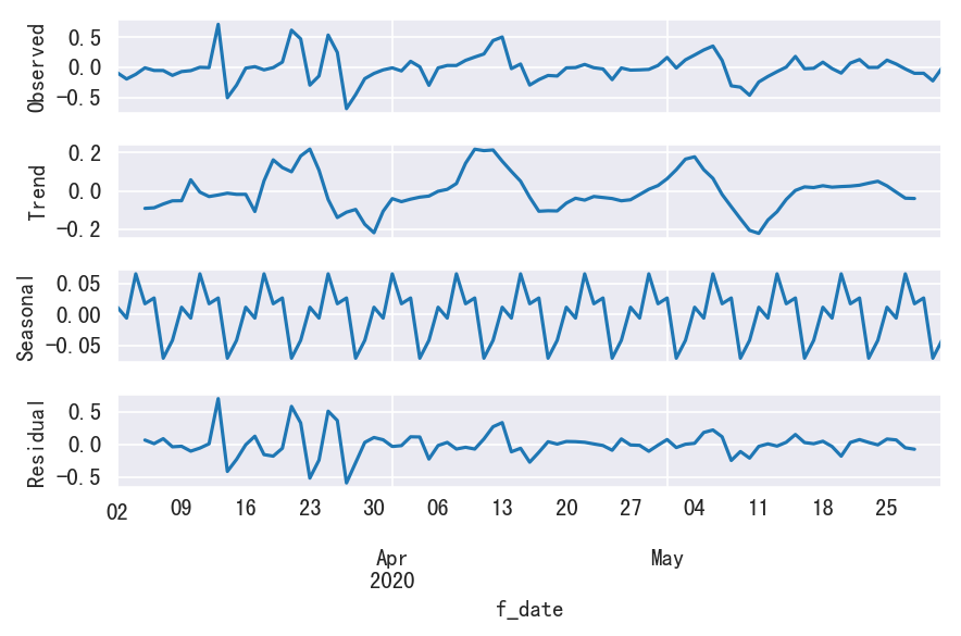
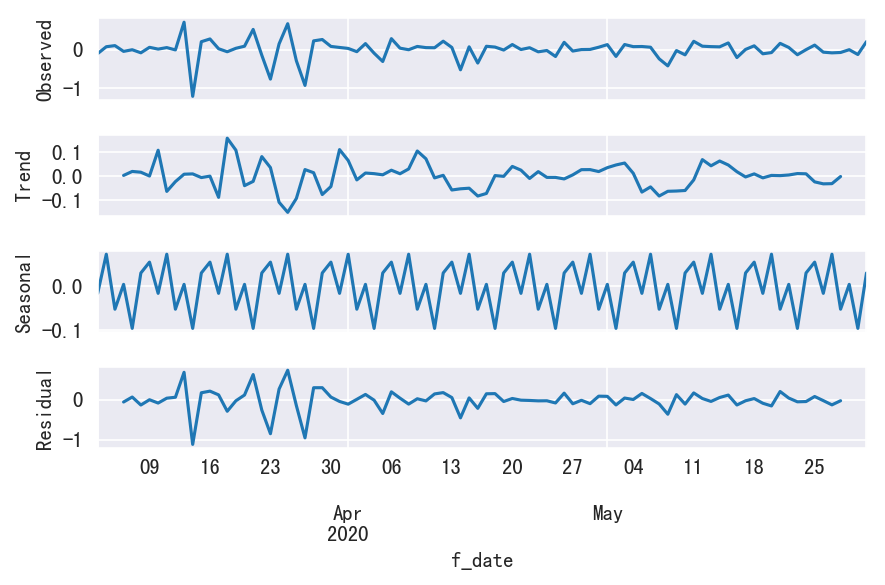
1 | season_resolve(s_dau_new_log_diff) |
test: p=0.0
(-5.650643581278351, 9.878845977099614e-07, 9, 75, {'5%': -2.9009249540740742, '1%': -3.520713130074074, '10%': -2.5877813777777776}, -88.7065598940126)
Test Statistic                -5.65
p-value                        0.00
#Lags Used                     9.00
Number of Observations Used   75.00
Critical Value (5%)           -2.90
Critical Value (1%)           -3.52
Critical Value (10%)          -2.59
dtype: float64
数据是否平稳(1/0): 1
1 | season_resolve(s_dau_new_log_diff2) |
test: p=0.0
(-5.898783625957804, 2.8100827285187457e-07, 11, 72, {'5%': -2.9026070739026064, '1%': -3.524624466842421, '10%': -2.5886785262345677}, -68.75760108315257)
Test Statistic                -5.90
p-value                        0.00
#Lags Used                    11.00
Number of Observations Used   72.00
Critical Value (5%)           -2.90
Critical Value (1%)           -3.52
Critical Value (10%)          -2.59
dtype: float64
数据是否平稳(1/0): 1
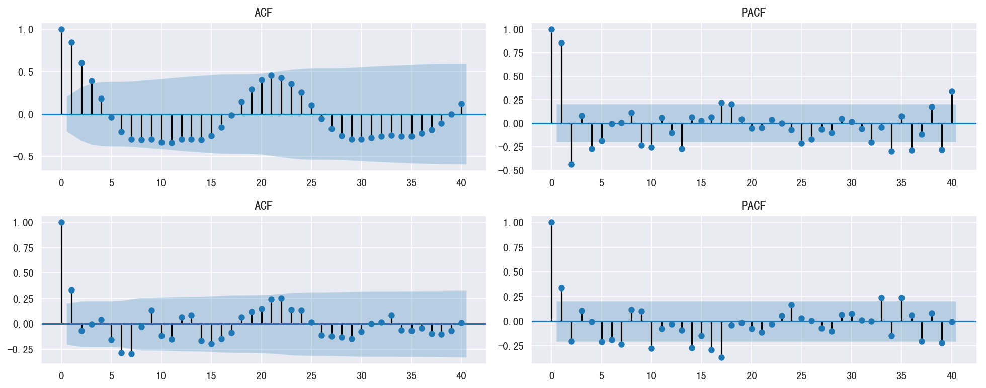
自相关图
1 | def plot_acf_pacf(df_list): |
1 | plot_acf_pacf([s_dau_new_log, s_dau_new_log_diff]) |
网格搜索
1 | def parameter_selection(df, ps=[0,1,2], ds=[2], qs=[0,1,2]): |
1 | matrix = parameter_selection(s_dau_new_log, ps=range(4), qs=range(4)) |
(0, 2, 0) - BIC:15.5504937045
(0, 2, 1) - BIC:-3.90439313959
(0, 2, 2) - BIC:-16.7008738132
(1, 2, 0) - BIC:13.7741898435
(1, 2, 1) - BIC:-13.1288961798
(1, 2, 2) - BIC:-14.7089870806
(1, 2, 3) - BIC:-13.2074940281
(2, 2, 0) - BIC:0.12566262446
(2, 2, 1) - BIC:-14.3782928385
(2, 2, 2) - BIC:-13.0656053424
(2, 2, 3) - BIC:-13.1196434498
(3, 2, 0) - BIC:-1.77302826664
(3, 2, 1) - BIC:-13.5275309286
(3, 2, 2) - BIC:-10.9182600295
(3, 2, 3) - BIC:-10.6767970671
最优参数:x(0, 2, 2) - AIC:-16.7008738132
1 | def max_node(p, d, q, P, D, Q, s): |
1 | pdq = [0, 2, 2] |
x(0, 0, 0, 7) - AIC:-15.9235194034 need 10 observations
x(0, 0, 1, 7) - AIC:-14.7113328488 need 25 observations
x(0, 0, 2, 7) - AIC:-29.4064147183 need 46 observations
x(0, 1, 0, 7) - AIC:63.48723362 need 17 observations
x(0, 1, 1, 7) - AIC:-2.14367734565 need 32 observations
x(0, 1, 2, 7) - AIC:-11.8848525187 need 53 observations
x(0, 2, 0, 7) - AIC:141.898368919 need 24 observations
x(0, 2, 1, 7) - AIC:39.8814708492 need 39 observations
x(0, 2, 2, 7) - AIC:2.67172770386 need 60 observations
x(1, 0, 0, 7) - AIC:-13.7461303101 need 10 observations
x(1, 0, 1, 7) - AIC:-13.4284053199 need 25 observations
x(1, 0, 2, 7) - AIC:-30.6083506043 need 46 observations
x(1, 1, 0, 7) - AIC:26.5931599614 need 17 observations
x(1, 1, 1, 7) - AIC:11.54952856 need 32 observations
x(1, 1, 2, 7) - AIC:-11.5907261101 need 53 observations
x(1, 2, 0, 7) - AIC:79.078108805 need 24 observations
x(1, 2, 1, 7) - AIC:47.7740298619 need 39 observations
x(1, 2, 2, 7) - AIC:6.90057268677 need 60 observations
x(2, 0, 0, 7) - AIC:-41.7769269787 need 17 observations
x(2, 0, 1, 7) - AIC:-40.1960951619 need 25 observations
x(2, 0, 2, 7) - AIC:-37.2401608236 need 46 observations
x(2, 1, 0, 7) - AIC:-9.33829251277 need 24 observations
x(2, 1, 1, 7) - AIC:-19.2066580221 need 32 observations
x(2, 1, 2, 7) - AIC:-22.4909020767 need 53 observations
x(2, 2, 0, 7) - AIC:25.240615073 need 31 observations
x(2, 2, 1, 7) - AIC:18.7858056712 need 39 observations
x(2, 2, 2, 7) - AIC:11.9538869508 need 60 observations
x(3, 0, 0, 7) - AIC:-38.0001167775 need 24 observations
x(3, 0, 1, 7) - AIC:-45.2099169457 need 25 observations
x(3, 0, 2, 7) - AIC:-49.2523157208 need 46 observations
x(3, 1, 0, 7) - AIC:-32.9888239169 need 31 observations
x(3, 1, 1, 7) - AIC:-31.4343836764 need 32 observations
x(3, 1, 2, 7) - AIC:-30.8665326957 need 53 observations
x(3, 2, 0, 7) - AIC:8.55482266627 need 38 observations
x(3, 2, 1, 7) - AIC:-4.72304771546 need 39 observations
x(3, 2, 2, 7) - AIC:-3.35845958847 need 60 observations
最优参数:x(3, 0, 2, 7) - AIC:-49.2523157208
1 | pred_dau_arima = myets.arima(train=myets.s_dau_new, |
RMSE=0.078732475591

1 | df_show(pred_dau_arima_diff.loc[pred_start_date: pred_end_date], 0, 14).dropna() |
shape=(10, 4)
| f_dau_new_origin | f_dau_new_predict | f_dau_new_diff | f_dau_new_rate | |
|---|---|---|---|---|
| f_date | ||||
| 2020-06-01 | 588936.00 | 566249.56 | -22686.44 | -0.04 |
| 2020-06-02 | 507322.00 | 529802.47 | 22480.47 | 0.04 |
| 2020-06-03 | 459898.00 | 516113.69 | 56215.69 | 0.12 |
| 2020-06-04 | 434520.00 | 486794.93 | 52274.93 | 0.12 |
| 2020-06-05 | 440420.00 | 451129.71 | 10709.71 | 0.02 |
| 2020-06-06 | 419283.00 | 455463.38 | 36180.38 | 0.09 |
| 2020-06-07 | 409955.00 | 433574.34 | 23619.34 | 0.06 |
| 2020-06-08 | 422092.00 | 398749.40 | -23342.60 | -0.06 |
| 2020-06-09 | 412235.00 | 374202.33 | -38032.67 | -0.09 |
ETS
1 | pred_dau_new = myets.pred_dau_new(trend='add', |
RMSE=0.0654776482142
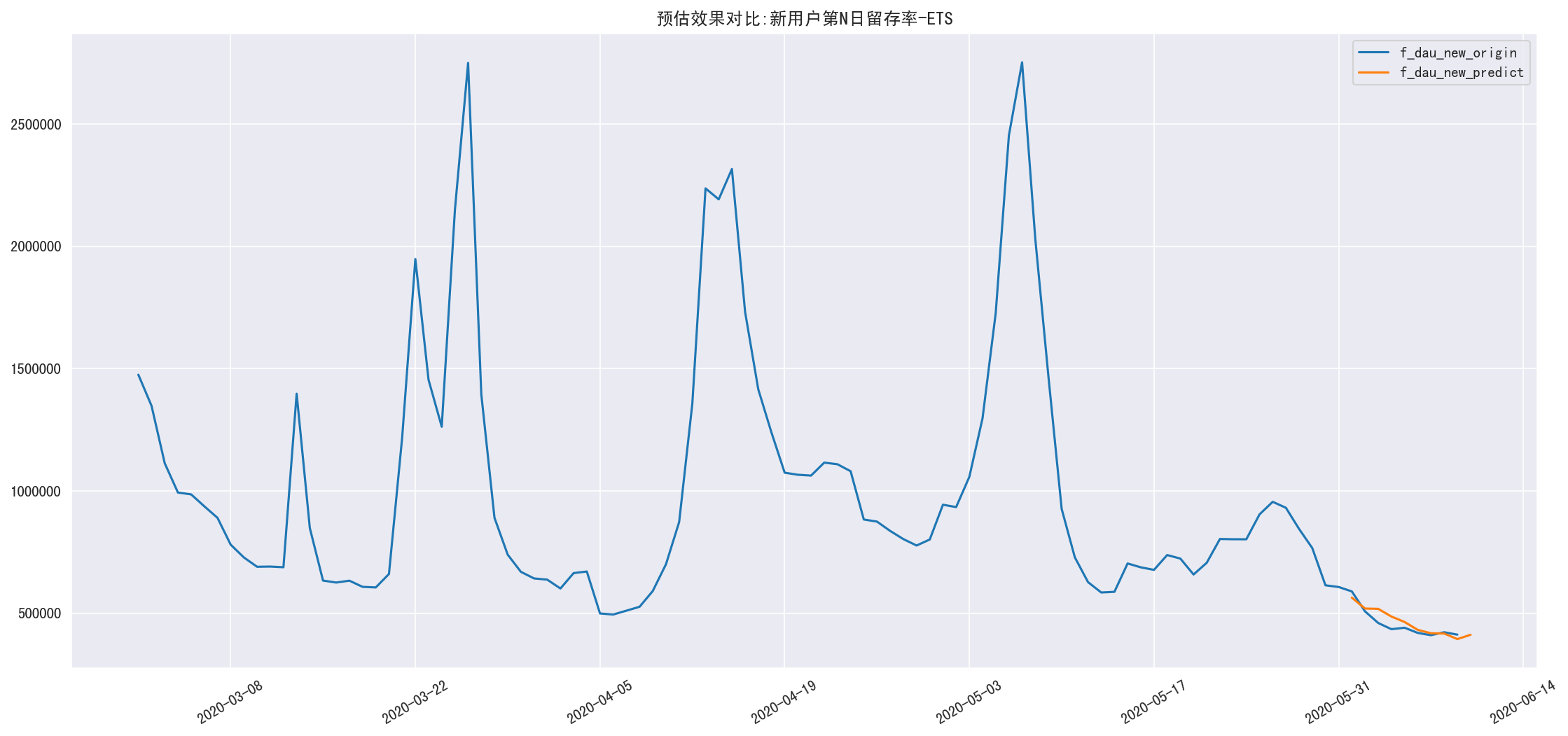
1 | df_show(pred_dau_new_diff.loc[pred_start_date: pred_end_date],0,14).dropna() |
shape=(10, 4)
| f_dau_new_origin | f_dau_new_predict | f_dau_new_diff | f_dau_new_rate | |
|---|---|---|---|---|
| 2020-06-01 | 588936.00 | 563557.69 | -25378.31 | -0.04 |
| 2020-06-02 | 507322.00 | 518941.51 | 11619.51 | 0.02 |
| 2020-06-03 | 459898.00 | 517735.65 | 57837.65 | 0.13 |
| 2020-06-04 | 434520.00 | 486268.62 | 51748.62 | 0.12 |
| 2020-06-05 | 440420.00 | 463959.35 | 23539.35 | 0.05 |
| 2020-06-06 | 419283.00 | 431672.77 | 12389.77 | 0.03 |
| 2020-06-07 | 409955.00 | 417944.87 | 7989.87 | 0.02 |
| 2020-06-08 | 422092.00 | 416701.86 | -5390.14 | -0.01 |
| 2020-06-09 | 412235.00 | 394114.05 | -18120.95 | -0.04 |
新用户留存
1 | df_show(df_ret_new,3,10) |
shape=(160, 120)
| f_remain_days | 1 | 2 | 3 | 4 | 5 | 6 | 7 | 8 | 9 | 10 | ... | 111 | 112 | 113 | 114 | 115 | 116 | 117 | 118 | 119 | 120 |
|---|---|---|---|---|---|---|---|---|---|---|---|---|---|---|---|---|---|---|---|---|---|
| f_visit_day | |||||||||||||||||||||
| 2020-01-01 | 0.02 | 0.01 | 0.01 | 0.01 | 0.01 | 0.01 | 0.01 | 0.01 | 0.00 | 0.01 | ... | 0.01 | 0.01 | 0.01 | 0.01 | 0.01 | 0.01 | 0.01 | 0.01 | 0.01 | 0.01 |
| 2020-01-02 | 0.02 | 0.01 | 0.01 | 0.01 | 0.01 | 0.01 | 0.01 | 0.01 | 0.01 | 0.01 | ... | 0.01 | 0.01 | 0.01 | 0.01 | 0.01 | 0.01 | 0.01 | 0.01 | 0.01 | 0.01 |
| 2020-01-03 | 0.02 | 0.01 | 0.01 | 0.01 | 0.01 | 0.01 | 0.01 | 0.01 | 0.01 | 0.01 | ... | 0.01 | 0.01 | 0.01 | 0.01 | 0.01 | 0.01 | 0.01 | 0.01 | 0.01 | 0.01 |
| 2020-05-30 | 0.11 | 0.05 | 0.03 | 0.02 | 0.01 | 0.01 | 0.01 | 0.01 | 0.01 | 0.01 | ... | nan | nan | nan | nan | nan | nan | nan | nan | nan | nan |
| 2020-05-31 | 0.07 | 0.03 | 0.02 | 0.01 | 0.01 | 0.01 | 0.01 | 0.01 | 0.01 | nan | ... | nan | nan | nan | nan | nan | nan | nan | nan | nan | nan |
| 2020-06-01 | 0.06 | 0.03 | 0.02 | 0.01 | 0.01 | 0.01 | 0.01 | 0.01 | nan | nan | ... | nan | nan | nan | nan | nan | nan | nan | nan | nan | nan |
| 2020-06-02 | 0.05 | 0.02 | 0.02 | 0.01 | 0.01 | 0.01 | 0.01 | nan | nan | nan | ... | nan | nan | nan | nan | nan | nan | nan | nan | nan | nan |
| 2020-06-03 | 0.05 | 0.02 | 0.01 | 0.01 | 0.01 | 0.01 | nan | nan | nan | nan | ... | nan | nan | nan | nan | nan | nan | nan | nan | nan | nan |
| 2020-06-04 | 0.04 | 0.02 | 0.01 | 0.01 | 0.01 | nan | nan | nan | nan | nan | ... | nan | nan | nan | nan | nan | nan | nan | nan | nan | nan |
| 2020-06-05 | 0.04 | 0.02 | 0.01 | 0.01 | nan | nan | nan | nan | nan | nan | ... | nan | nan | nan | nan | nan | nan | nan | nan | nan | nan |
| 2020-06-06 | 0.03 | 0.02 | 0.01 | nan | nan | nan | nan | nan | nan | nan | ... | nan | nan | nan | nan | nan | nan | nan | nan | nan | nan |
| 2020-06-07 | 0.03 | 0.02 | nan | nan | nan | nan | nan | nan | nan | nan | ... | nan | nan | nan | nan | nan | nan | nan | nan | nan | nan |
| 2020-06-08 | 0.04 | nan | nan | nan | nan | nan | nan | nan | nan | nan | ... | nan | nan | nan | nan | nan | nan | nan | nan | nan | nan |
13 rows × 120 columns
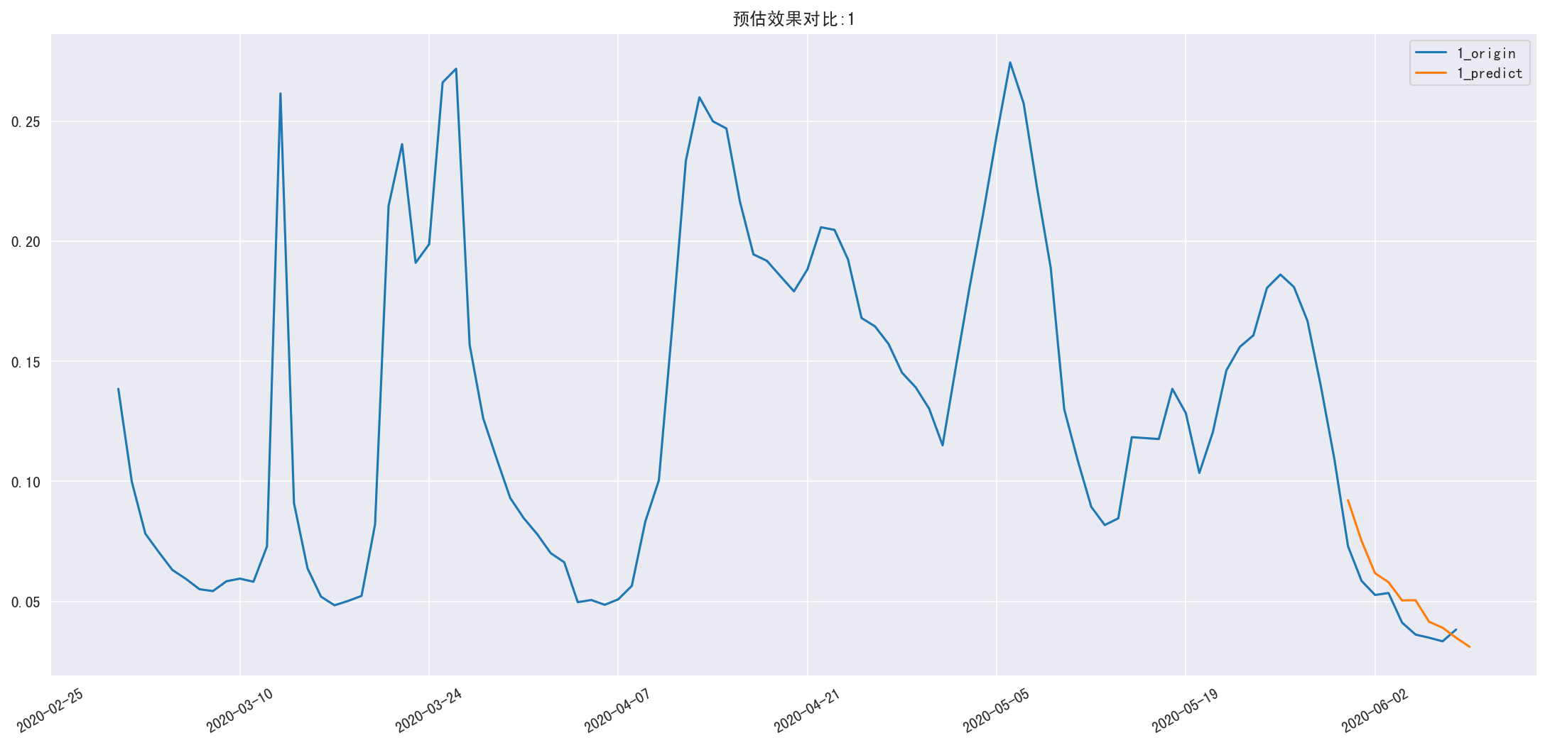
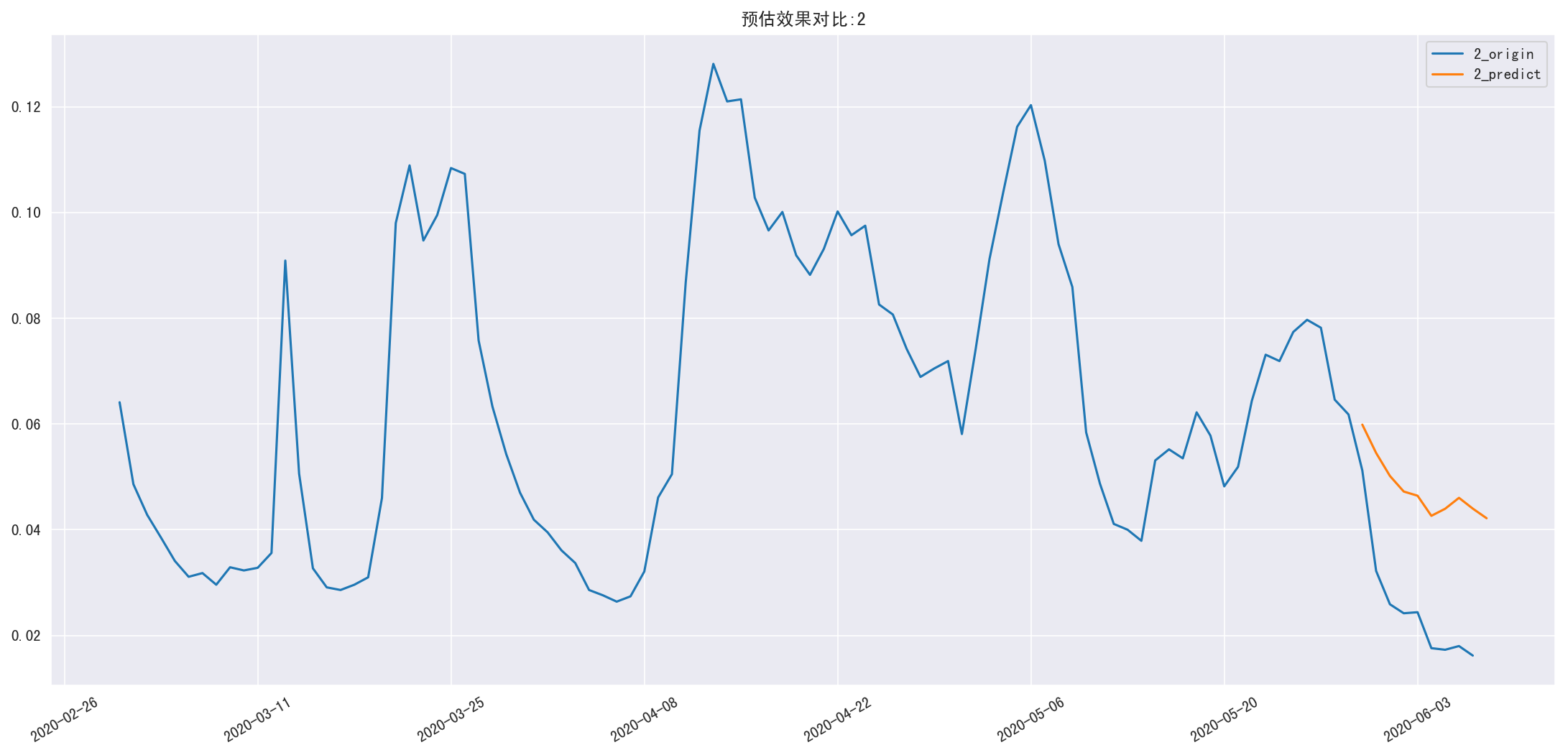
新用户第 N 日留存预估
1 | def predict_ret_new_n(n): |
RMSE=0.227393637754
RMSE=1.19606960639
新用户第 N 日留存预估矩阵
1 | pred_ret_new_ratio = myets.pred_ret_new(trend=None, |
1 | df_show(pred_ret_new_ratio,3,15) |
shape=(102, 102)
| 0 | 1 | 2 | 3 | 4 | 5 | 6 | 7 | 8 | 9 | ... | 92 | 93 | 94 | 95 | 96 | 97 | 98 | 99 | 100 | 101 | |
|---|---|---|---|---|---|---|---|---|---|---|---|---|---|---|---|---|---|---|---|---|---|
| 2020-03-01 | 1 | 0.14 | 0.06 | 0.04 | 0.03 | 0.02 | 0.02 | 0.02 | 0.02 | 0.01 | ... | 0.00 | 0.00 | 0.00 | 0.00 | 0.01 | 0.00 | 0.01 | 0.01 | 0.00 | 0.00 |
| 2020-03-02 | 1 | 0.10 | 0.05 | 0.03 | 0.03 | 0.02 | 0.02 | 0.02 | 0.01 | 0.01 | ... | 0.01 | 0.01 | 0.01 | 0.01 | 0.01 | 0.01 | 0.01 | 0.01 | 0.01 | nan |
| 2020-03-03 | 1 | 0.08 | 0.04 | 0.03 | 0.02 | 0.02 | 0.02 | 0.02 | 0.02 | 0.01 | ... | 0.01 | 0.01 | 0.00 | 0.00 | 0.00 | 0.00 | 0.01 | 0.01 | nan | nan |
| 2020-05-27 | 1 | 0.18 | 0.08 | 0.04 | 0.02 | 0.02 | 0.01 | 0.01 | 0.01 | 0.01 | ... | nan | nan | nan | nan | nan | nan | nan | nan | nan | nan |
| 2020-05-28 | 1 | 0.17 | 0.06 | 0.03 | 0.03 | 0.02 | 0.02 | 0.01 | 0.01 | 0.01 | ... | nan | nan | nan | nan | nan | nan | nan | nan | nan | nan |
| 2020-05-29 | 1 | 0.14 | 0.06 | 0.04 | 0.03 | 0.02 | 0.02 | 0.01 | 0.01 | 0.01 | ... | nan | nan | nan | nan | nan | nan | nan | nan | nan | nan |
| 2020-05-30 | 1 | 0.11 | 0.07 | 0.04 | 0.03 | 0.02 | 0.02 | 0.01 | 0.01 | 0.01 | ... | nan | nan | nan | nan | nan | nan | nan | nan | nan | nan |
| 2020-05-31 | 1 | 0.11 | 0.06 | 0.04 | 0.03 | 0.02 | 0.01 | 0.01 | 0.01 | 0.01 | ... | nan | nan | nan | nan | nan | nan | nan | nan | nan | nan |
| 2020-06-01 | 1 | 0.11 | 0.06 | 0.04 | 0.03 | 0.02 | 0.01 | 0.01 | 0.01 | 0.01 | ... | nan | nan | nan | nan | nan | nan | nan | nan | nan | nan |
| 2020-06-02 | 1 | 0.11 | 0.06 | 0.04 | 0.02 | 0.02 | 0.01 | 0.01 | 0.01 | nan | ... | nan | nan | nan | nan | nan | nan | nan | nan | nan | nan |
| 2020-06-03 | 1 | 0.11 | 0.06 | 0.03 | 0.02 | 0.02 | 0.01 | 0.01 | nan | nan | ... | nan | nan | nan | nan | nan | nan | nan | nan | nan | nan |
| 2020-06-04 | 1 | 0.11 | 0.06 | 0.03 | 0.03 | 0.02 | 0.02 | nan | nan | nan | ... | nan | nan | nan | nan | nan | nan | nan | nan | nan | nan |
| 2020-06-05 | 1 | 0.12 | 0.06 | 0.04 | 0.03 | 0.02 | nan | nan | nan | nan | ... | nan | nan | nan | nan | nan | nan | nan | nan | nan | nan |
| 2020-06-06 | 1 | 0.11 | 0.07 | 0.04 | 0.03 | nan | nan | nan | nan | nan | ... | nan | nan | nan | nan | nan | nan | nan | nan | nan | nan |
| 2020-06-07 | 1 | 0.11 | 0.06 | 0.04 | nan | nan | nan | nan | nan | nan | ... | nan | nan | nan | nan | nan | nan | nan | nan | nan | nan |
| 2020-06-08 | 1 | 0.11 | 0.06 | nan | nan | nan | nan | nan | nan | nan | ... | nan | nan | nan | nan | nan | nan | nan | nan | nan | nan |
| 2020-06-09 | 1 | 0.11 | nan | nan | nan | nan | nan | nan | nan | nan | ... | nan | nan | nan | nan | nan | nan | nan | nan | nan | nan |
| 2020-06-10 | 1 | nan | nan | nan | nan | nan | nan | nan | nan | nan | ... | nan | nan | nan | nan | nan | nan | nan | nan | nan | nan |
18 rows × 102 columns
老用户留存
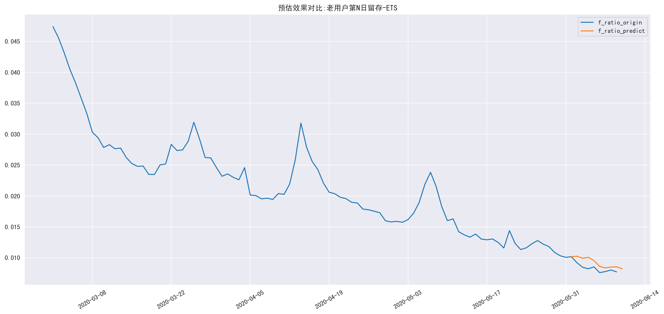
老用户第 N 日留存率预估
1 | # 转置 |
RMSE=0.127854181665
1 | df_show(pred_ret_old_result,0,15) |
shape=(102, 4)
| f_ratio_origin | f_ratio_predict | f_ratio_diff | f_ratio_rate | |
|---|---|---|---|---|
| f_date | ||||
| 2020-05-27 | 0.01 | nan | nan | nan |
| 2020-05-28 | 0.01 | nan | nan | nan |
| 2020-05-29 | 0.01 | nan | nan | nan |
| 2020-05-30 | 0.01 | nan | nan | nan |
| 2020-05-31 | 0.01 | nan | nan | nan |
| 2020-06-01 | 0.01 | 0.01 | 0.00 | 0.00 |
| 2020-06-02 | 0.01 | 0.01 | 0.00 | 0.12 |
| 2020-06-03 | 0.01 | 0.01 | 0.00 | 0.17 |
| 2020-06-04 | 0.01 | 0.01 | 0.00 | 0.23 |
| 2020-06-05 | 0.01 | 0.01 | 0.00 | 0.12 |
| 2020-06-06 | 0.01 | 0.01 | 0.00 | 0.13 |
| 2020-06-07 | 0.01 | 0.01 | 0.00 | 0.08 |
| 2020-06-08 | 0.01 | 0.01 | 0.00 | 0.06 |
| 2020-06-09 | 0.01 | 0.01 | 0.00 | 0.11 |
| 2020-06-10 | nan | 0.01 | nan | nan |
新老用户留存率矩阵
1 | # 备份修改 |
| 0 | 1 | 2 | 3 | 4 | 5 | 6 | 7 | 8 | 9 | ... | 93 | 94 | 95 | 96 | 97 | 98 | 99 | 100 | 101 | 102 | |
|---|---|---|---|---|---|---|---|---|---|---|---|---|---|---|---|---|---|---|---|---|---|
| 2020-02-29 | 1.00 | 0.05 | 0.05 | 0.04 | 0.04 | 0.04 | 0.04 | 0.03 | 0.03 | 0.03 | ... | 0.01 | 0.01 | 0.01 | 0.01 | 0.01 | 0.01 | 0.01 | 0.01 | 0.01 | 0.01 |
1 rows × 103 columns
1 | ratio_matrix = pd.concat([pred_ret_old_ratio, pred_ret_new_ratio]).sort_index().sort_index(axis=1) |
shape=(103, 103)
| 0 | 1 | 2 | 3 | 4 | 5 | 6 | 7 | 8 | 9 | ... | 93 | 94 | 95 | 96 | 97 | 98 | 99 | 100 | 101 | 102 | |
|---|---|---|---|---|---|---|---|---|---|---|---|---|---|---|---|---|---|---|---|---|---|
| 2020-02-29 | 1.00 | 0.05 | 0.05 | 0.04 | 0.04 | 0.04 | 0.04 | 0.03 | 0.03 | 0.03 | ... | 0.01 | 0.01 | 0.01 | 0.01 | 0.01 | 0.01 | 0.01 | 0.01 | 0.01 | 0.01 |
| 2020-03-01 | 1.00 | 0.14 | 0.06 | 0.04 | 0.03 | 0.02 | 0.02 | 0.02 | 0.02 | 0.01 | ... | 0.00 | 0.00 | 0.00 | 0.01 | 0.00 | 0.01 | 0.01 | 0.00 | 0.00 | nan |
| 2020-03-02 | 1.00 | 0.10 | 0.05 | 0.03 | 0.03 | 0.02 | 0.02 | 0.02 | 0.01 | 0.01 | ... | 0.01 | 0.01 | 0.01 | 0.01 | 0.01 | 0.01 | 0.01 | 0.01 | nan | nan |
| 2020-03-03 | 1.00 | 0.08 | 0.04 | 0.03 | 0.02 | 0.02 | 0.02 | 0.02 | 0.02 | 0.01 | ... | 0.01 | 0.00 | 0.00 | 0.00 | 0.00 | 0.01 | 0.01 | nan | nan | nan |
| 2020-03-04 | 1.00 | 0.07 | 0.04 | 0.03 | 0.02 | 0.02 | 0.02 | 0.02 | 0.01 | 0.01 | ... | 0.01 | 0.00 | 0.00 | 0.01 | 0.01 | 0.01 | nan | nan | nan | nan |
| 2020-03-05 | 1.00 | 0.06 | 0.03 | 0.02 | 0.02 | 0.02 | 0.02 | 0.02 | 0.01 | 0.01 | ... | 0.01 | 0.00 | 0.01 | 0.01 | 0.01 | nan | nan | nan | nan | nan |
| 2020-03-06 | 1.00 | 0.06 | 0.03 | 0.02 | 0.02 | 0.02 | 0.02 | 0.02 | 0.01 | 0.01 | ... | 0.00 | 0.00 | 0.01 | 0.01 | nan | nan | nan | nan | nan | nan |
| 2020-03-07 | 1.00 | 0.06 | 0.03 | 0.02 | 0.02 | 0.02 | 0.02 | 0.01 | 0.01 | 0.01 | ... | 0.01 | 0.00 | 0.00 | nan | nan | nan | nan | nan | nan | nan |
| 2020-03-08 | 1.00 | 0.05 | 0.03 | 0.02 | 0.02 | 0.02 | 0.02 | 0.01 | 0.01 | 0.01 | ... | 0.00 | 0.00 | nan | nan | nan | nan | nan | nan | nan | nan |
| 2020-03-09 | 1.00 | 0.06 | 0.03 | 0.02 | 0.02 | 0.02 | 0.02 | 0.02 | 0.01 | 0.01 | ... | 0.01 | nan | nan | nan | nan | nan | nan | nan | nan | nan |
| 2020-06-01 | 1.00 | 0.11 | 0.06 | 0.04 | 0.03 | 0.02 | 0.01 | 0.01 | 0.01 | 0.01 | ... | nan | nan | nan | nan | nan | nan | nan | nan | nan | nan |
| 2020-06-02 | 1.00 | 0.11 | 0.06 | 0.04 | 0.02 | 0.02 | 0.01 | 0.01 | 0.01 | nan | ... | nan | nan | nan | nan | nan | nan | nan | nan | nan | nan |
| 2020-06-03 | 1.00 | 0.11 | 0.06 | 0.03 | 0.02 | 0.02 | 0.01 | 0.01 | nan | nan | ... | nan | nan | nan | nan | nan | nan | nan | nan | nan | nan |
| 2020-06-04 | 1.00 | 0.11 | 0.06 | 0.03 | 0.03 | 0.02 | 0.02 | nan | nan | nan | ... | nan | nan | nan | nan | nan | nan | nan | nan | nan | nan |
| 2020-06-05 | 1.00 | 0.12 | 0.06 | 0.04 | 0.03 | 0.02 | nan | nan | nan | nan | ... | nan | nan | nan | nan | nan | nan | nan | nan | nan | nan |
| 2020-06-06 | 1.00 | 0.11 | 0.07 | 0.04 | 0.03 | nan | nan | nan | nan | nan | ... | nan | nan | nan | nan | nan | nan | nan | nan | nan | nan |
| 2020-06-07 | 1.00 | 0.11 | 0.06 | 0.04 | nan | nan | nan | nan | nan | nan | ... | nan | nan | nan | nan | nan | nan | nan | nan | nan | nan |
| 2020-06-08 | 1.00 | 0.11 | 0.06 | nan | nan | nan | nan | nan | nan | nan | ... | nan | nan | nan | nan | nan | nan | nan | nan | nan | nan |
| 2020-06-09 | 1.00 | 0.11 | nan | nan | nan | nan | nan | nan | nan | nan | ... | nan | nan | nan | nan | nan | nan | nan | nan | nan | nan |
| 2020-06-10 | 1.00 | nan | nan | nan | nan | nan | nan | nan | nan | nan | ... | nan | nan | nan | nan | nan | nan | nan | nan | nan | nan |
20 rows × 103 columns
DAU留存矩阵
1 | dau_matrix = ratio_matrix.mul(pred_dau_new, axis='index') |
shape=(103, 103)
| 0 | 1 | 2 | 3 | 4 | 5 | 6 | 7 | 8 | 9 | ... | 93 | 94 | 95 | 96 | 97 | 98 | 99 | 100 | 101 | 102 | |
|---|---|---|---|---|---|---|---|---|---|---|---|---|---|---|---|---|---|---|---|---|---|
| 2020-02-29 | 273385370.00 | 12958148.00 | 12452616.00 | 11797162.00 | 11073535.00 | 10472504.00 | 9798707.00 | 9117300.00 | 8284139.00 | 8039563.00 | ... | 2699356.59 | 2715180.35 | 2626011.84 | 2671154.75 | 2519520.16 | 2264857.58 | 2199788.72 | 2234150.08 | 2249973.83 | 2160805.32 |
| 2020-03-01 | 1475032.00 | 204291.93 | 94549.55 | 58411.27 | 43218.44 | 34663.25 | 29648.14 | 25223.05 | 22420.49 | 20650.45 | ... | 6936.95 | 5220.64 | 7032.82 | 7539.64 | 4889.92 | 7497.01 | 7614.17 | 7092.76 | 7053.06 | nan |
| 2020-03-02 | 1347642.00 | 134494.67 | 65495.40 | 44202.66 | 34364.87 | 27896.19 | 23448.97 | 21966.56 | 19675.57 | 18866.99 | ... | 9554.92 | 9098.68 | 9092.78 | 8151.67 | 6763.07 | 11073.35 | 9959.14 | 9417.70 | nan | nan |
| 2020-03-03 | 1112908.00 | 87029.41 | 47632.46 | 33943.69 | 26932.37 | 21924.29 | 20700.09 | 18362.98 | 17917.82 | 16359.75 | ... | 6765.79 | 4993.47 | 4390.72 | 4932.99 | 4972.60 | 7680.72 | 7071.00 | nan | nan | nan |
| 2020-03-04 | 993211.00 | 70021.38 | 38238.62 | 27015.34 | 20956.75 | 19268.29 | 16785.27 | 16189.34 | 14798.84 | 14600.20 | ... | 6376.45 | 3963.54 | 4519.98 | 5838.69 | 5006.08 | 7176.47 | nan | nan | nan | nan |
| 2020-03-05 | 985703.00 | 62197.86 | 33612.47 | 23065.45 | 20206.91 | 17348.37 | 16559.81 | 14982.69 | 14588.40 | 12814.14 | ... | 6147.21 | 4536.31 | 6059.73 | 6628.64 | 5874.86 | nan | nan | nan | nan | nan |
| 2020-03-06 | 936955.00 | 55655.13 | 29139.30 | 22955.40 | 18739.10 | 17146.28 | 15272.37 | 14991.28 | 13304.76 | 11993.02 | ... | 4524.75 | 3964.23 | 4799.75 | 5515.87 | nan | nan | nan | nan | nan | nan |
| 2020-03-07 | 889821.00 | 49029.14 | 28296.31 | 20821.81 | 17618.46 | 15304.92 | 14593.06 | 13169.35 | 11834.62 | 11389.71 | ... | 4509.68 | 3406.76 | 4220.58 | nan | nan | nan | nan | nan | nan | nan |
| 2020-03-08 | 780080.00 | 42358.34 | 23090.37 | 17629.81 | 14821.52 | 13573.39 | 12013.23 | 10999.13 | 10219.05 | 9594.98 | ... | 3668.65 | 2760.97 | nan | nan | nan | nan | nan | nan | nan | nan |
| 2020-03-09 | 727798.00 | 42503.40 | 23944.55 | 17903.83 | 15429.32 | 12809.24 | 11353.65 | 11062.53 | 10261.95 | 9461.37 | ... | 5160.16 | nan | nan | nan | nan | nan | nan | nan | nan | nan |
| 2020-06-01 | 563557.69 | 62103.07 | 35575.73 | 20969.61 | 14305.90 | 10089.09 | 7795.20 | 6727.99 | 5750.08 | 5095.59 | ... | nan | nan | nan | nan | nan | nan | nan | nan | nan | nan |
| 2020-06-02 | 518941.51 | 56246.99 | 32305.73 | 19031.49 | 12288.68 | 9177.43 | 7599.00 | 6267.09 | 5469.77 | nan | ... | nan | nan | nan | nan | nan | nan | nan | nan | nan | nan |
| 2020-06-03 | 517735.65 | 58635.20 | 32593.13 | 18076.83 | 12242.16 | 9718.19 | 7724.17 | 6392.72 | nan | nan | ... | nan | nan | nan | nan | nan | nan | nan | nan | nan | nan |
| 2020-06-04 | 486268.62 | 54515.05 | 29297.18 | 17014.05 | 12271.39 | 9261.54 | 7372.38 | nan | nan | nan | ... | nan | nan | nan | nan | nan | nan | nan | nan | nan | nan |
| 2020-06-05 | 463959.35 | 54259.31 | 28966.35 | 17484.08 | 11792.88 | 8750.09 | nan | nan | nan | nan | ... | nan | nan | nan | nan | nan | nan | nan | nan | nan | nan |
| 2020-06-06 | 431672.77 | 48169.79 | 28347.88 | 16167.69 | 10923.33 | nan | nan | nan | nan | nan | ... | nan | nan | nan | nan | nan | nan | nan | nan | nan | nan |
| 2020-06-07 | 417944.87 | 47617.30 | 27000.65 | 15774.89 | nan | nan | nan | nan | nan | nan | ... | nan | nan | nan | nan | nan | nan | nan | nan | nan | nan |
| 2020-06-08 | 416701.86 | 45919.82 | 26305.16 | nan | nan | nan | nan | nan | nan | nan | ... | nan | nan | nan | nan | nan | nan | nan | nan | nan | nan |
| 2020-06-09 | 394114.05 | 42717.21 | nan | nan | nan | nan | nan | nan | nan | nan | ... | nan | nan | nan | nan | nan | nan | nan | nan | nan | nan |
| 2020-06-10 | 411632.31 | nan | nan | nan | nan | nan | nan | nan | nan | nan | ... | nan | nan | nan | nan | nan | nan | nan | nan | nan | nan |
20 rows × 103 columns
DAU 预估
1 | # df_result['ret_old'] = pd.Series(dau_matrix.loc[base_date-timedelta(1)].values, |
shape=(10, 6)
| dau_origin | dau_sum | dau_new | ret_old | ret_new | check | |
|---|---|---|---|---|---|---|
| 2020-06-01 | 3994272 | 3922560.87 | 563557.69 | 2699356.59 | 659646.59 | 0.00 |
| 2020-06-02 | 3546456 | 3925123.98 | 518941.51 | 2715180.35 | 691002.12 | 0.00 |
| 2020-06-03 | 3248834 | 3830069.65 | 517735.65 | 2626011.84 | 686322.16 | -0.00 |
| 2020-06-04 | 3129509 | 3864890.96 | 486268.62 | 2671154.75 | 707467.59 | 0.00 |
| 2020-06-05 | 3216982 | 3691592.09 | 463959.35 | 2519520.16 | 708112.58 | 0.00 |
| 2020-06-06 | 2895258 | 3331318.71 | 431672.77 | 2264857.58 | 634788.36 | 0.00 |
| 2020-06-07 | 2926685 | 3222451.35 | 417944.87 | 2199788.72 | 604717.76 | 0.00 |
| 2020-06-08 | 3023940 | 3298679.82 | 416701.86 | 2234150.08 | 647827.88 | -0.00 |
| 2020-06-09 | 2911481 | 3327172.93 | 394114.05 | 2249973.83 | 683085.04 | 0.00 |
| 2020-06-10 | 2737987 | 3258783.04 | 411632.31 | 2160805.32 | 686345.40 | 0.00 |
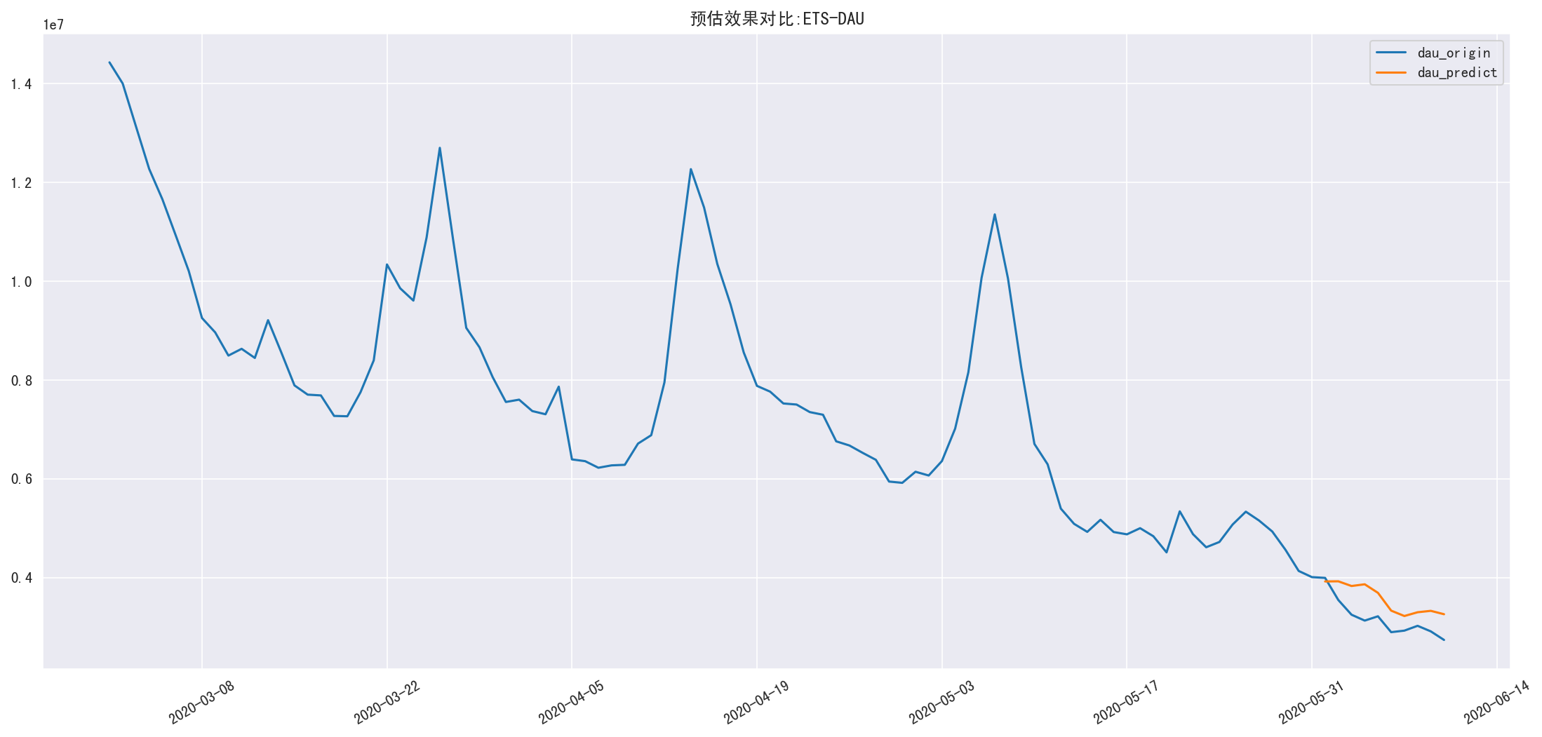
验证
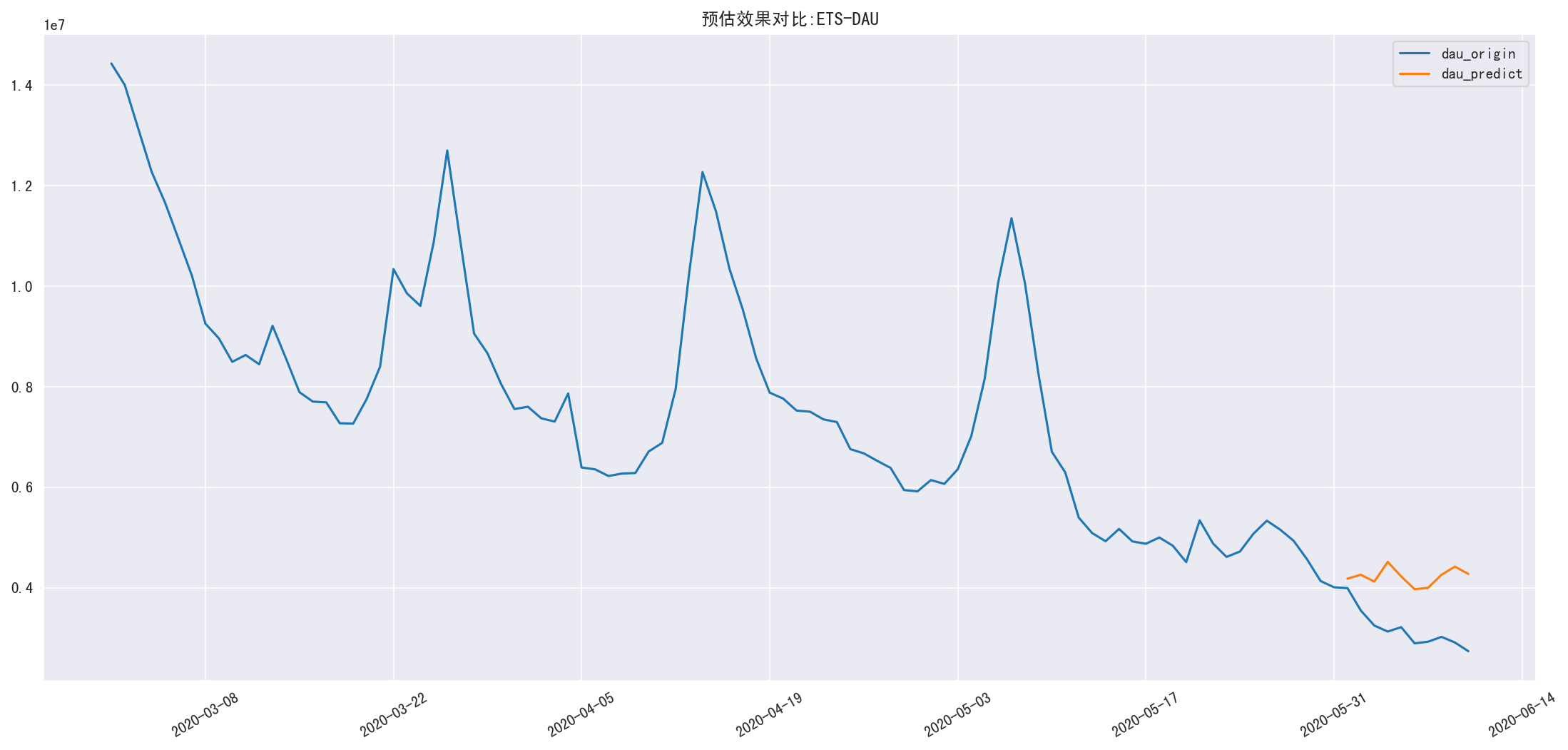
1 | result = myets.predict_compare(ets_result['dau_sum'], dau.loc['2020-03-01':], u'ETS-DAU') |
RMSE=0.147793852021
1 | arima_result = get_dau_arima() |
RMSE=0.378640685005